Asymptotic notation is a way to describe the behaviour of an algorithm as the input size grows indefinitely. It allows us to understand how the running time or space requirements of an algorithm change as the input size increases, which is useful for comparing the relative efficiency of different algorithms. In this blog post, we will cover the three main types of asymptotic notation: Big O, Big Ω, and Big Θ.

Big O Notation :

Big O notation is used to describe the upper bound on the running time or space requirements of an algorithm. It tells us the worst-case scenario for the algorithm's performance. For example, if an algorithm has a running time of O(n), this means that in the worst case running time grows linearly with the input size.

To understand this, let us consider the example of linear search. Suppose we want to find the number 3 in the following array:

Arr = {2,7,1,5,8,4,10,9,6,3}

Here, 3 is the last element, and we will find it in the last iteration using linear search. So, this is the worst-case scenario where the loop will run the maximum number of times. The run-time will also be the maximum value possible.

Linear search in Java:

public static int linearSearch(int[] arr, int target) {
    for (int i = 0; i < arr.length; i++) {
    if (arr[i] == target) {
        return i;
        }
    }
    return -1;
}

Big O notation is usually expressed as a mathematical function. Some common functions that are used in Big O notation include:

• O(1): Constant time. The running time of the algorithm does not depend on the input size.

• O(log n): Logarithmic time. The running time grows logarithmically with the input size. This is commonly seen in algorithms that divide the input size in half repeatedly, such as binary search.

• O(n): Linear time. The running time grows linearly with the input size.

• O(n log n): Linear logarithmic time. The running time grows as the input size is multiplied by the log of the input size. This is commonly seen in algorithms that divide and conquer, such as merge sort.

• O(n^2): Quadratic time. The running time grows as the square of the input size. This is commonly seen in algorithms that nest two loops, such as bubble sort.

• O(2^n): Exponential time. The running time grows exponentially with the input size. This is commonly seen in algorithms that generate all subsets of a set, such as the travelling salesman problem.

It's important to note that Big O notation is an upper bound, not a tight bound. This means that the actual running time of an algorithm might be faster than the bound suggested by the notation. For example, an algorithm with a running time of O(n^2) might have a running time closer to O(n) under certain circumstances.

In mathematical terms :

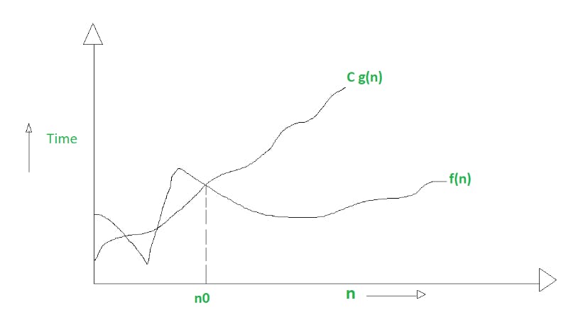
O(g(n)) = { f(n): there exist positive constants C and n0
            such that 0 ≤ f(n) ≤ Cg(n) for all n ≥ n0 }

Big Ω Notation :

Big Ω (also known as Big-Omega) notation is used to describe the lower bound on the running time or space requirements of an algorithm. It tells us the best-case scenario for the algorithm's performance.

To understand this, let us again consider our previous example. Again we want to find 3 using linear search, but the elements in the array will be in a different order.

Arr = {3,7,1,2,8,4,10,9,6,5}

As you can see, by linear search, we will find 3 in the very first iteration of the loop. So, this is the best-case scenario since the loop will run only once, and therefore the run-time will be the least possible.

In the above example, the complexity can never be less than the best-case complexity; therefore, the complexity in Big Ω notation will be Ω(1). In fact, the complexity in Big Ω for all algorithms is usually always Ω(1).

Big Ω notation is often used in conjunction with Big O notation to give a more complete picture of the performance of an algorithm. By understanding both the lower and upper bounds on the running time or space requirements of an algorithm, we can get a better idea of how the algorithm will perform in practice.

In mathematical terms :

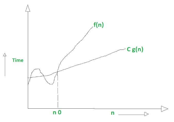
Ω(g(n)) = { f(n): there exist positive constants C and n0 
            such that 0 ≤ Cg(n) ≤ f(n) for all n ≥ n0 }

Big Θ Notation :

Big Θ (also known as Big-Theta) notation is used to describe the average-case or expected running time or space requirements of an algorithm. It is a combination of Big O and Big Ω notation, and it tells us the running time or space requirements of an algorithm under typical circumstances.

Let us again consider the same example but with the array elements arranged differently.

Arr = {2,7,1,3,5,8,4,10,9,6}

Here, the element we are searching for, 5, is present precisely in the middle. So, the complexity will be average in the case of linear search, and the run-time will be the average time taken.

Big Θ is either the algorithm’s exact performance value or a good range between narrow upper and lower bounds.

In mathematical terms :

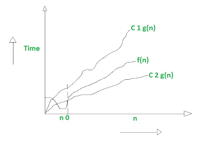
Θ(g(n)) = { f(n): there exist positive constants C1, C2 and n0
            such that 0 ≤ C2g(n) ≤ f(n) ≤ C1g(n) for all n ≥ n0 }

Asymptotic Analysis Example :

Now that we have covered the three main types of asymptotic notation, let's look at an example of how we can use asymptotic analysis to compare the efficiency of two different algorithms.

Suppose we have two algorithms for sorting a list of numbers:

• Algorithm A has a running time of O(2^n)

• Algorithm B has a running time of O(n^3)

At first glance, it might seem like Algorithm A is faster, since the running time grows more slowly with the input size. However, as the input size gets very large, the difference in performance becomes much more significant. For example, with an input size of 1000, Algorithm A takes more than 10^301 steps to complete, while Algorithm B takes only 10^9 steps.

To understand why this is the case, we can use asymptotic analysis to compare the growth rates of the two algorithms. The O(2^n) running time of Algorithm A grows much faster than the O(n^3) running time of Algorithm B, so even though Algorithm A has a lower running time for small input sizes, it becomes much slower as the input size increases.

In general, algorithms with a lower asymptotic running time or space requirement will be more efficient in the long run. However, it's important to keep in mind that asymptotic analysis is just a way to understand the long-term behaviour of an algorithm. It doesn't necessarily tell us how an algorithm will perform on a specific input or with a specific input size.

I hope this revised blog post helped explain the basics of asymptotic notation and analysis. Asymptotic notation is an important tool for understanding the efficiency of algorithms and comparing the relative performance of different approaches. It's an essential concept to understand when working with data structures and algorithms.